Understanding the Universal Approximation Theorem for single variable real valued functions

[Note: All of this code used in this post can be found at this colab link, but with a slightly different exposition.]

Universal Approximation Theorems are fundamental results in the mathematics of machine learning.

One of the best ways to understand a theorem is to try and prove it yourself. In turn, one of the best ways to try to prove a hard theorem is to strip away as much complexity as possible and attempt to prove the simplest possible version you can. This is what this post attempts to accomplish: to show, from scratch, how to approximate any continuous function \(f: [x_1,x_2] \to \mathbb{R}\) using a feed-forward neural network with unbounded width.

Let’s unpack that a little.

The simplest feed-forward neural network is a function from \(\mathbb{R} \to \mathbb{R}\) defined by

where \(W: \mathbb{R} \to \mathbb{R}^n\) is a linear map, \(b \in \mathbb{R}^n\) is a vector, \(\textrm{relu}(x) = \textrm{ max}(0,x)\) (applied to each coordinate), and \(C:\mathbb{R}^n \to \mathbb{R}\) is another linear map.

Our goal is to show that given any continuous function \(f: [x_1,x_2] \to \mathbb{R}\), we can find \(n, C, W, b\) so that the corresponding neural network approximates \(f\) to a desired degree of accuracy with respect to some norm on the function space.

We can set up all of this machinery in python pretty easily:

import numpy as np

def relu(x):
    return np.maximum(0,x)

def hidden_layer(C, W,b):
    return lambda x: np.dot(C,relu(np.dot(W,x)+b))[0,0]

Notice that \(\textrm{hidden_layer(C, W,b)}: \mathbb{R} \to \mathbb{R}\) can be thought of as a sum of the transformed relus:

The \(C_i, W_i\), and \(b_i\) are vertically stretching, horizontally stretching, and horizontally shifting the \(\textrm{relu}\) function around.

As an example, let’s compute a hidden_layer which I will call slant_step (for reasons which will become apparent) with

then we have

The graph of \(- \textrm{ relu}(x - 1)\) can be obtained from the graph of relu by shifting to the right horizontally by 1 and then reflecting over the horizontal axis. So the graph of slant_step is obtained by adding the graph of relu and this shifted and reflected relu.

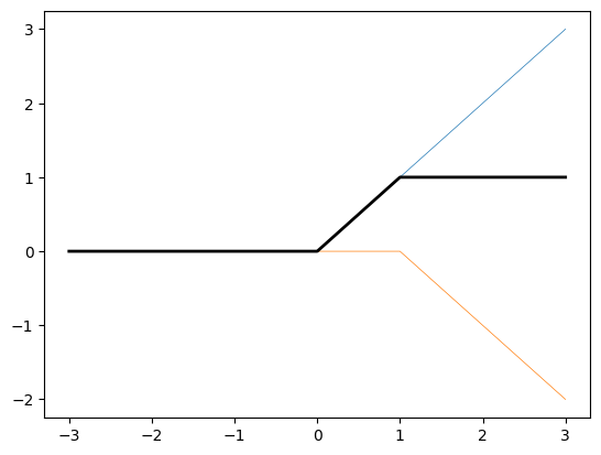
We can confirm that slant_step has the following formula by case analysis:

slant_step will be important to us because stretching and translating this example can give us a small “rise” over however long of a “run” we want, while being constant elsewhere. Summing lots of these will give us piecewise linear approximations to any function we like!

In particular

is the function

Also note that it is easy to represent a non-zero constant function in the form \(\textrm{hidden_layer}(C,W,b)\). If we want our constant to be \(k\) just take \(b = \mid k \mid\), \(W = 0\), and \(C = \frac{b}{\mid b \mid}\). To represent the constant \(0\) function we just take all of them to be zero.

Finally, we can represent the pointwise sum of the functions \(\textrm{hidden_layer}(C_1,W_1,b_1)\) and \(\textrm{hidden_layer}(C_2,W_2,b_2)\) as maps \(\mathbb{R} \to \mathbb{R}\) by using

where I am using horizontal or vertical juxtoposition to denote concatenation along the indicated axis.

Putting it all together we can approximate any continuous function \(f: [x_1, x_2] \to \mathbb{R}\) using a single \(\textrm{hidden_layer}\). The \(\textrm{hidden_layer}\) we build will be a piecewise linear interpolation of \(f\). We will:

• Partition \([x_1,x_2]\) into \(N\) equal-sized subintervals of width \(\textrm{run} = \frac{x_2 - x_1}{N}\).
• Start with the hidden_layer for the constant function \(x \mapsto f(x_1)\)
• For \(i = 0, 1, 2, ..., N - 1\):
  • Compute \(\textrm{slope}_i\) of the secant line over the \(i^{th}\) subinteveral.
  • Use this to find \(C_i, W_i, b_i\) for the transformed slant_step function which is \(0\) to the left of the \(i^{th}\) subinteveral, has slope \(\textrm{slope}_i\) over the \(i^{th}\) subinteveral, and is constant to the right.
• Concatenate the \(C_i, W_i, b_i\) to give the pointwise sum of all of these.

Here is some python code which accomplishes this:

def universal_approx_theorem(f,x1,x2,N):
    # The initial C, W, b represent a constant hidden_layer with value f(x1).
    C = np.array([[np.sign(f(x1))]])
    W = np.array([[0]])
    b = np.array([[np.absolute(f(x1))]])
    run = (x2-x1)/N
    for i in range(N):
        start = x1 + i*run
        stop = x1 + (i+1)*run
        rise = f(stop) - f(start)
        slope = rise/run
        # concatenating along the appropriate axis is equivalent to summing the corresponding hidden layers as functions R -> R.
        # At each iteration we are adding a slant_step which goes from 0 at the left endpoint of the
        # subinterval to "rise" at the right endpoint of the subinterval.
        # The resulting hidden_layer is linear on each subinterval and interpolates f on the partition points.
        C = np.concatenate((C, np.array([[slope, -slope]])), axis = 1)
        W = np.concatenate((W, np.array([[1],[1]])), axis = 0)
        b = np.concatenate((b, np.array([[-start],[-stop]])), axis = 0)
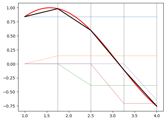
    return (C,W,b)

To help visualize this, we can look at how 4 slant_step functions sum up to a piecewise linear approximation of sine

Let’s contrast this with the kind of approximation that we could find by training a neural network. We are using a dense layer of dimension \(1 + 2\cdot 4 = 9\) to match the dimension of the approximation we computed above.

import tensorflow as tf
import keras
from keras import layers

X = np.linspace(1, 4, 1000)
y = np.sin(X)

model = keras.Sequential([
    layers.Dense(9, activation = 'relu', use_bias = True ,input_shape=(1,)),
    layers.Dense(1)
])

model.compile(optimizer = "rmsprop",
              loss = "mse",
              metrics = ["mean_squared_error"])

model.fit(X, y, epochs = 200)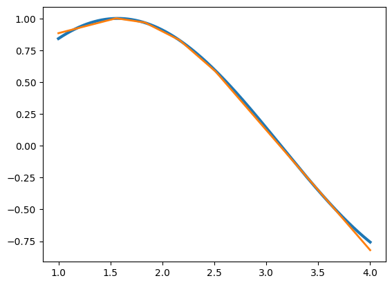

We can see that compared to the hidden_layer algorithm, the neural network was able to get 5 subintervals (better than our 4), and also tailored the size of these subintervals to be smaller over regions with more curvature and larger over regions with less curvature. I will note that running this code did not always produce such a good approximation though! Interestingly it seems that if the initial random selection of weights resulted in a line, the algorithm converged to a local minimum of the loss function which just fit a line with no subdivisions (i.e. we ended up just doing linear regression). It is interesting to think about whether starting with algorithmically generated weights like the ones we found for universal_approx_theorem would be a better starting configuration for training than if we started with random weights.

For fun here is our universal_approx_theorem using 100 subdivisions (i.e. a hidden layer of dimension 201) along with all of the shifted and scaled slant_step functions which are being summed.

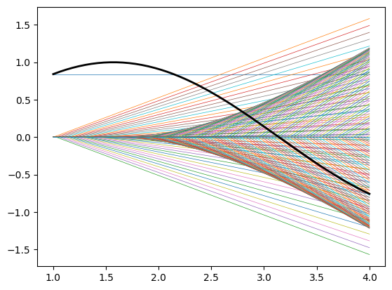
The cool payoff here is that we have

where \(C\) is a 201 dimensional co-vector and \(W\) and \(b\) are both 201 dimensional vectors. The matrix \(b\) is recording the partitition of the interval, \(W\) is doing basically nothing, and \(C\) is recording the slopes of the piecewise linear approximations.