In this post we:
- Motivate and gain some geometric understanding of the Singular Value Decomposition.
- Give a formal proof that the SVD exists which follows the geometric intuition.
- Gain some geometric intuition for \(X^\top X\) and how to connect the SVD with the eigenstuff of \(X^\top X\).
- How to use SVD to do linear regression (aka projecting a vector \(\vec{y}\) onto \(\textrm{Im}(X)\)).
- See how the SVD naturally gives best low rank approximations of linear transformations.
- Understand the subspace similarity metric introduced in the LoRa paper through the geometric lens we have developed here.
Geometric Motivation for SVD
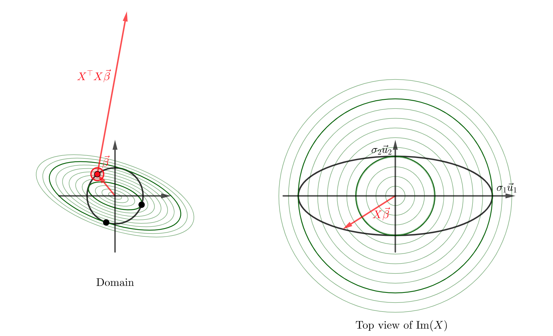
Consider the matrix
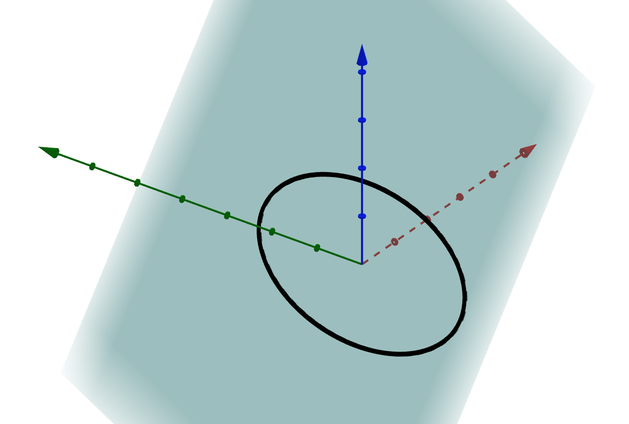
\[X = \begin{bmatrix} 1 & 1 \\ 1& 3 \\ 1 & -1\end{bmatrix}\]Then the image of \(X\) is the plane spanned by the columns of \(X\).
The image of the unit circle is an ellipse.
You can access an interactive version here.
The singular value decomposition of \(X\) is motivated by a compelling geometric problem: we want to find the axes of this ellipse.
For now let’s just treat the SVD as a black box, and see each part of the SVD corresponds to a part of the solution to this problem.
import numpy as np

X = np.array([[1,1],[1,3],[1, -1]])
svdstuff = np.linalg.svd(X)

U = svdstuff[0]

D = np.concatenate([np.diag(svdstuff[1]), np.zeros((1,2))])

V = np.transpose(svdstuff[2])
print('U = \n', U)
print('\n D = \n', D)
print('\n V = \n', V)

print('\n These should be equal \n',  X, '\n = \n ', np.dot(U, np.dot(D, np.transpose(V))))
U = [[-3.65148372e-01 4.47213595e-01 -8.16496581e-01] [-9.12870929e-01 -2.57661936e-16 4.08248290e-01] [ 1.82574186e-01 8.94427191e-01 4.08248290e-01]]
D = [[3.46410162 0. ] [0. 1.41421356] [0. 0. ]]
V = [[-0.31622777 0.9486833 ] [-0.9486833 -0.31622777]]
These should be equal [[ 1 1] [ 1 3] [ 1 -1]] = [[ 1. 1.] [ 1. 3.] [ 1. -1.]]
So we have
\[X = U \Sigma V^\top\]with
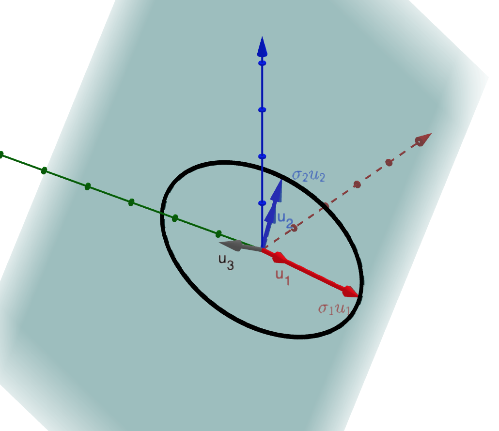
\[U \approx \begin{bmatrix} 0.365 & 0.447 & -8.16 \\ -0.912 & 0 & -0.408\\ 0.182 & -.894 & 0.402 \end{bmatrix} \hphantom{dsds} \Sigma \approx \begin{bmatrix} 3.464 & 0 \\ 0 & 1.414 \\ 0 & 0 \end{bmatrix} \hphantom{dsds} V \approx \begin{bmatrix} -0.316 & 0.949 \\ -0.949 & -0.316 \end{bmatrix}\]The columns of \(U\), which we call the left singular vectors are
\[\vec{u}_1 = \begin{bmatrix} 0.365 \\ -0.912 \\ 0.182 \end{bmatrix} \hphantom{dsds} \vec{u}_2 = \begin{bmatrix} 0.447 \\ 0 \\ -.894 \end{bmatrix} \hphantom{dsds} \vec{u}_3 = \begin{bmatrix} -0.816 \\ 0.408\\ 0.402 \end{bmatrix}\]The diagaonl entries of \(\Sigma\) are \(\sigma_1 = 3.464\) and \(\sigma_2 = 1.414\).
Let’s visualize what we have so far before moving on to \(V\):
Again, you can access an interactive version here.
We can see that \(\vec{u}_1\) is the unit vector pointing in the direction of the major axis of the ellipse, \(\vec{u}_2\) is the unit vector pointing in the direction of the minor axis of the ellipse, and \(\vec{u}_3\) is just chosen to complete an orthonormal basis of the codomain.
\(\sigma_1 \vec{u}_1\) and \(\sigma_2 \vec{u}_2\) are the vectors pointing from the center of the ellipse to the vertexes of the ellipse. \(\sigma_1\) and \(\sigma_2\) are the lengths of these.
The columns of \(V\), which we call the right singular vectors are
\[\vec{v}_1 = \begin{bmatrix} -0.316 \\ -0.949 \end{bmatrix} \hphantom{dsds} \vec{v}_2 = \begin{bmatrix} 0.949 \\ -0.316 \end{bmatrix}\]Let’s plot these in the domain:
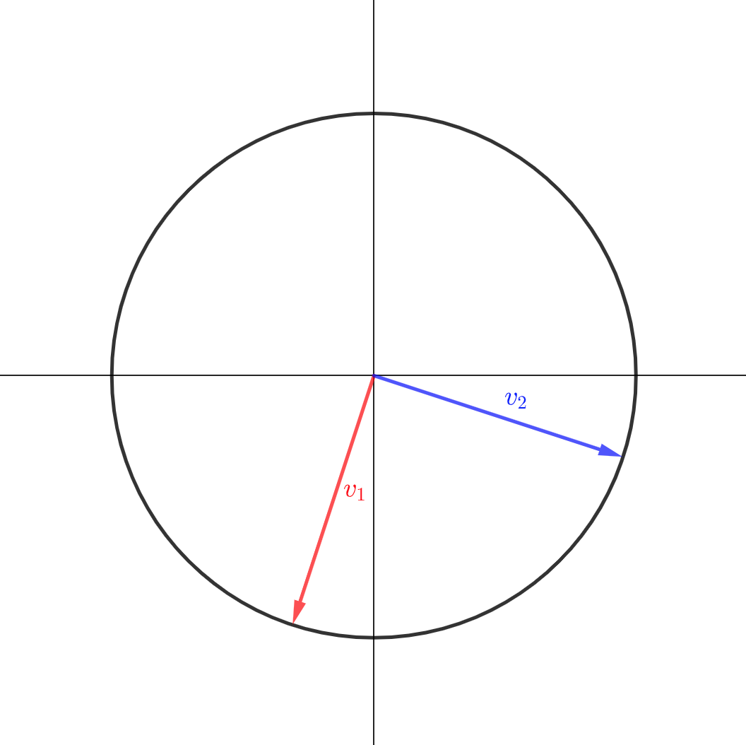
These have been chosen so that
\[\begin{align*} X \vec{v}_1 = \sigma_1 \vec{u}_1\\ X \vec{v}_2 = \sigma_2 \vec{u}_2 \end{align*}\]In other words the right singular vectors (the \(\vec{v}_j\)) are the inverse images of the vertexes of the ellipse.
You may not have noticed it but a small miracle has occured. The right singular vectors are orthogonal to each other! This is really the key insight which makes SVD possible. We will understand why this happens soon.
To summarize, and slightly generalize:
- We started with a \(n \times p\) matrix \(X\).
- The unit sphere in \(\mathbb{R}^p\) is transformed into an ellipsoid living in \(\textrm{Im}(X)\) in the domain \(\mathbb{R}^n\).
- Let \(r = \textrm{Rank}(X)\). We found the unit vectors \(\vec{u}_1, \vec{u}_2, \dots, \vec{u}_r\) pointing in the direction of the axes of this ellipsoid. We let \(\sigma_1, \sigma_2, \dots \sigma_r\) be the distance from the origin to these vertexes.
- \(\vec{v}_1, \vec{v}_2 , \dots \vec{v}_r\) are chosen to be inverse images of \(\sigma_1 \vec{u}_1, \sigma_2\vec{u}_2, \dots, \sigma_r \vec{u}_r\). It is a small miracle that these end up orthogonal as well.
- If \(n > r\), then we also completed the \(u_j\) to form a basis of \(\mathbb{R}^n\): \(\vec{u}_{r+1}, \vec{u}_{r+2}, \dots \vec{u}_n\) are chosen to be orthonormal and span \(\textrm{Im}(X)^\perp\).
- Similarly, if \(p > r\) then the null space of \(X\) will be \(\textrm{Span}(\vec{v}_1, \vec{v}_2 , \dots \vec{v}_r)^\perp\), and we choose the remaining \(v_j\) to complete an orthonormal basis of \(\mathbb{R}^p\). You could also view this as the image ellipsoid having “degenerate axes” of length \(0\), and extend the \(\sigma_j\) to be \(0\) in this case.
- At the end of this process we have orthonormal bases of both the domain and codomain with:
Let’s attempt to carry out this construction in general.
To find the major axis we will maximize \(S(\beta) = \left\vert X \vec{\beta} \right\vert^2\) subject to the constraint that \(g(\beta) = \left\vert \vec{\beta} \right\vert^2 = 1\). Note that the maximum must exist because \(S\) is a continuous function which we are maximizing a continuous function on the unit sphere in \(\mathbb{R}^n\) which is compact. So we know that the maximum value is achieved.
To do this we will use the method of Lagrange Multipliers: at the maximizing \(\vec{\beta}_{\textrm{max}}\) we have
\[\nabla S \big \vert_{\vec{\beta}_{\textrm{max}}} = \lambda \nabla g\big \vert_{\vec{\beta}_{\textrm{max}}}\]You can find a full explanation of how to compute these gradients here: just set \(\vec{y} = \vec{0}\) in that derivation.
We have
\[\nabla S \big \vert_{\vec{\beta}} = 2 X^\top X \vec{\beta} \hphantom{dsds} \nabla g \big \vert_{\vec{\beta}} = 2\vec{\beta}\]so we have that
\[X^\top X \vec{\beta}_{\textrm{max}} = \lambda \vec{\beta}_{\textrm{max}}\]Notice that this also implies (apply \(\vec{\beta}_{\textrm{max}}^\top\) to both sides) that \(\vert X \vec{\beta}_{\textrm{max}}\vert^2 = \lambda\), so \(\lambda \geq 0\).
The key to SVD is the following lemma, which explains the small miracle we observed in our concrete example:
Small Miracle Lemma:
Let \(X\), \(\lambda\), \(\vec{\beta}_{\textrm{max}}\) be as above. Let \(\vec{\beta}_\textrm{perp}\) be any vector orthogonal to \(\vec{\beta}_{\textrm{max}}\). Then \(X\vec{\beta}_\textrm{perp}\) is also orthogonal to \(X \vec{\beta}_\textrm{max}\).
Proof:
\[\begin{align*} \langle X\vec{\vec{\beta}}_\textrm{perp}, X \vec{\beta}_\textrm{max} \rangle &= \langle \vec{\beta}_\textrm{perp}, X^\top X \vec{\beta}_\textrm{max} \rangle \\ &= \langle \vec{\beta}_\textrm{perp}, \lambda \vec{\beta}_\textrm{max} \rangle \\ &= \lambda \langle \vec{\beta}_\textrm{perp}, \vec{\beta}_\textrm{max} \rangle \\ &= 0 \end{align*}\]This lemma has a nice geometric interpretation: \(\vec{\beta}_{\textrm{max}}\) is a radial vector of the unit sphere, and \(\vec{\beta}_{\textrm{perp}}\) is perpendicular to it. For a sphere, the tangent space is the space of vectors perpendicular to the radial vector. In the codomain we are looking at an ellipsoid. In general a radial vector will not be perpendicular to the tangent space of the ellipsoid, but we are saying it is when that radial vector is along the major axis of the ellipse.
Adjust the value of the slider \(s\) in this geogebra link. You can see that the radial vector of an ellipse is only perpendicular to the tangent line at the axes of the ellipse.
This should be geometrically reasonable: at points where the radial vector and tangent line are not perpendicular, the radial vector will get a little bigger if moved one direction, and a little smaller if moved in the other direction. At the max moving in either direction will increase the length, which means that the tangent line must be perpendicular to the radial vector.
We can now build bases for the domain and codomain of a matrix \(n \times p\) matrix \(X\) as follows:
- Choose \(\vec{v}_1\) to be a vector maximizing \(\vert X \vec{v_1}\vert^2\) subject to the constraint \(\vert\vec{v}_1\vert^2 = 1\). We have \(\vert X\vec{v}_1\vert^2 = \lambda_1\). Set \(\sigma_1 = \sqrt{\lambda_1}\), so that \(\vert X\vec{v}_1\vert = \sigma_1\).
- Set \(\vec{u}_1\) to be the unit vector pointing in the same direction as \(X \vec{v}_1\). By our computation, \(X \vec{v}_1 = \sigma_1 \vec{u}_1\).
- Now restrict the domain of \(X\) to \(\vec{v}_1^\perp\). By the lemma, the image of \(X \big \vert_{\vec{v}_1^\perp}\) is perpendicular to \(\vec{v}_1\). So we can iterate: choose \(\vec{v}_2\) to be a vector from \(\vec{v}_1^\perp\) subject to the constraint that \(\vert\vec{v}_2\vert^2 = 1\). We have \(\vert X\vec{v}_2\vert^2 = \lambda_2\). Set \(\sigma_2 = \sqrt{\lambda_2}\), so that \(\vert X\vec{v}_2\vert = \sigma_2\).
- Set \(\vec{u}_2\) to be the unit vector pointing in the same direction as \(X \vec{v}_2\), so that \(X \vec{v}_2 = \sigma_2 \vec{u}_2\). By the lemma \(\vec{u}_2 \perp \vec{u}_1\).
- Let \(r = \textrm{Rank}(X)\). Continue to iteratively construct orthonormal vectors \(\vec{v}_1,\vec{v_2},\vec{v_3}, \dots, \vec{v}_r\) and \(\vec{u}_1,\vec{u_2},\vec{u_3}, \dots, \vec{u}_r\) until the \(\vec{u}_j\) span the image of \(X\).
- At this point \(\textrm{Span}(\vec{v}_j)^\perp\) will be the null space of \(X\). We can find an orthonormal basis \(\vec{v}_{r+1}, \vec{v}_{r+2}, \vec{v}_{r+3}, \dots, \vec{v}_p\) of the null space. Similarly, we can find an orthonormal basis \(\vec{u}_{r+1}, \vec{u}_{r+2}, \dots, \vec{u}_{n}\) of \(\textrm{Im}(X)^\perp\). We can set \(\sigma_j = 0\) for \(j > \textrm{Rank}(X)\) so that we continue to have \(X \vec{v}_j = \sigma_j \vec{u}_j\) in this case.
- Now \(\{\vec{v}_j\}\) is an orthonormal basis of \(\mathbb{R}^p\), \(\{\vec{u}_j\}\) is an orthonormal basis of \(\mathbb{R}^n\), and we have
If we let \(U\) be the orthogonal matrix whose columns are \(\vec{u}_j\), \(V\) be the orthogonal matrix whose columns are \(\vec{v}_j\), and \(\Sigma\) be the \(n \times p\) matrix whose diagonal is \(\Sigma_{jj} = \sigma_j\), then we can rephrase this as the matrix factorization:
\[X = U \Sigma V^\top\]- Note: We call \(\vec{u}_j\) the left singular vectors, and \(\vec{v}_j\) the right singular vectors.
We have just proven the Singular Value Decomposition theorem. Let’s state it again formally:
Singular Value Decomposotion Theorem: Let \(X\) be any \(n \times p\) matrix. Then we can find a factorization \(X = U \Sigma V^\top\) where
- \(V\) is an orthogonal \(p \times p\) matrix (its columns form an orthonormal basis of \(\mathbb{R}^p\)).
- \(U\) is an orthogonal \(n \times n\) matrix (its columns form an orthonormal basis of \(\mathbb{R}^n\)).
- \(\Sigma\) is a \(n \times p\) matrix which has zero entries everywhere but the diagonal \(\Sigma_{jj} = \sigma_j \geq 0\).
Note: there are several slight variants of the SVD. One we will use in this post is the “compact SVD”. Here we only take the \(r = \textrm{Rank}(X)\) left and right singular vectors with non-zero singular values. So we get the decomposition
\[X = U_r \Sigma_r V_r^\top\]where \(V_r\) is an \(p \times r\) matrix, \(\Sigma_r\) is an \(r \times r\) diagonal matrix with positive values along the diagonal, and \(U_r\) is an \(n \times r\) matrix.
Understanding how our “basis building” intuition corresponds to the matrix factorization.
I think it is worth breaking down the expression
\[X = U \Sigma V^\top\]to really understand what each part is doing. I will “reconstruct” this formula using the basis vectors we found in the proof.
Let \(\vec{\beta}\) be any vector in \(\mathbb{R}^p\).
Since the \(\vec{v}_j\) form an orthonormal basis of \(\mathbb{R}^p\), it is easy to express \(\vec{\beta}\) in this basis: we just have
\[\vec{\beta} = (\vec{v}_1 \cdot \vec{\beta}) \vec{v_1} + (\vec{v}_2 \cdot \vec{\beta}) \vec{v_2} + \dots + (\vec{v}_p \cdot \vec{\beta}) \vec{v_p}\]We can compute the vector of coefficients using \(V^\top\):
\[\begin{align*} \begin{bmatrix} \vec{v}_1 \cdot \vec{\beta} \\ \vec{v}_2 \cdot \vec{\beta} \\ \vdots\\ \vec{v}_p \cdot \vec{\beta} \\ \end{bmatrix} &= \begin{bmatrix} \vec{v}_1^\top \vec{\beta} \\ \vec{v}_2^\top \vec{\beta} \\ \vdots\\ \vec{v}_p^\top \vec{\beta} \\ \end{bmatrix}\\ &= \begin{bmatrix} - & \vec{v}_1^\top & - \\ - & \vec{v}_2^\top & - \\ \vdots & \vdots & \vdots \\ - & \vec{v}_p^\top & - \\ \end{bmatrix} \vec{\beta}\\ &= V^\top \vec{\beta} \end{align*}\]If we apply \(X\) to \(\vec{\beta}\) expressed in this basis we get
\[\begin{align*} X(\vec{\beta}) &= X (\vec{v}_1 \cdot \vec{\beta}) \vec{v_1} + (\vec{v}_2 \cdot \vec{\beta}) \vec{v_2} + \dots + (\vec{v}_p \cdot \vec{\beta}) \vec{v_p} \\ &= (\vec{v}_1 \cdot \vec{\beta}) X(\vec{v_1}) + (\vec{v}_2 \cdot \vec{\beta}) X(\vec{v_2}) + \dots + (\vec{v}_p \cdot \vec{\beta}) X(\vec{v_p}) \\ &= \sigma_1(\vec{v}_1 \cdot \vec{\beta}) \vec{u_1} + \sigma_2(\vec{v}_1 \cdot \vec{\beta}) \vec{u_2} + \dots + \sigma_p(\vec{v}_p \cdot \vec{\beta}) \vec{u_p} + 0 \vec{u}_{p+1} + \dots + 0 \vec{u}_n\\ \end{align*}\]We already computed that the “vector of coefficients of \(\vec{\beta}\) when expressed in the basis of right singular vectors” was \(V^\top \vec{\beta}\).
We can see that we need to multiply these coefficients by \(\sigma_j\). The coefficients are now \(\Sigma V^\top \vec{\beta}\) (where \(\Sigma\) is also taking care of ``padding out’’ any extra \(0\) coefficients which may be needed).
We then want to use these coefficients to make a linear combination of the \(\vec{u}_j\). We do that just by writing \(U\Sigma V^\top\vec{\beta}\).
So we can see that for every \(\vec{\beta}\) we have
\[X\vec{\beta} = U\Sigma V^\top \vec{\beta}\]which is why we have the equality
\[X = U\Sigma V^\top\]In summary:
- \(V^\top \vec{\beta}\) records the coefficients of \(\vec{\beta}\) when written in the basis of \(\vec{v}_j\).
- \(\Sigma V^\top \vec{\beta}\) then scales these coefficients by the singular values, and pads the list with zeros at the end to match the dimension of the output space.
- \(U \Sigma V^\top \vec{\beta}\) uses the scaled coefficients to form a linear combination of the \(\vec{u}_j\).
- This is exactly what we want, since our understanding is that \(\vec{v}_j \mapsto \sigma_j \vec{u}_j\)!
Intuition for \(X^\top X\) and why the eigenstuff of \(X^\top X\) relates to the Singular Value Decompostion.
You may have noticed that in our proof of the small miracle lemma, ended up with
\[X^\top X \vec{\beta}_{\textrm{max}} = \lambda \vec{\beta}_{\textrm{max}}\]Another way to phrase this is that \(\vec{\beta}_{\textrm{max}}\) is an eigenvector for \(X^\top X\) with eigenvalue \(\lambda\). Since we obtained our singular value decomposition by repeatedly applying this lemma, it turns out that all of the right singular vectors are eigenvectors of \(X^\top X\). We can actually compute that pretty easily:
\[\begin{align*} X^\top X \vec{v}_j &= X^\top (\sigma_j \vec{u}_j)\\ &= (U \Sigma V^\top)^\top (\sigma_j \vec{u}_j)\\ &= V \Sigma^\top U^\top (\sigma_j \vec{u}_j)\\ &= \sigma_j V \Sigma^\top \vec{e}_j \textrm{ since $U$ is orthogonal, the only component which lives is the $j^{th}$ one.}\\ &= \sigma_j^2 V \vec{e}_j\\ &= \sigma_j^2 \vec{v}_j \end{align*}\]Note: I am using \(\vec{e}_j\) to represent the vector in \(\mathbb{R}^n\) with component \(1\) in the \(j^{th}\) coordinate and \(0\) otherwise.
This computation doesn’t give us a lot of intuition about \(X^\top X\) or why its eigenstuff should related to the SVD stuff of \(X\) though. What does \(X^\top X \vec{\beta}\) actually mean? Where is the connection to the ellipsoid?
The key to understanding \(X^\top X\) is the following fact. For any two vectors \(\vec{\beta}_1, \vec{\beta}_2 \in \mathbb{R}^p\), we have
\[\langle X^\top X \vec{\beta}_1, \vec{\beta}_2\rangle = \langle X \vec{\beta}_1, X\vec{\beta}_2\rangle\]This is important enough to turn into a slogan:
To compute the inner product of the images of two vectors \(\vec{\beta}_1\) and \(\vec{\beta}_2\) under the transformation \(X\), you can compute the inner product of \(\vec{\beta}_2\) with \(X^\top X \vec{\beta}_1\).
So \(X^\top X\) is a tool for understanding inner product stuff in \(\textrm{Im(X)}\) by representing it as inner product stuff happening in the domain.
Let’s make that concrete with an example.
Let’s choose our old friend
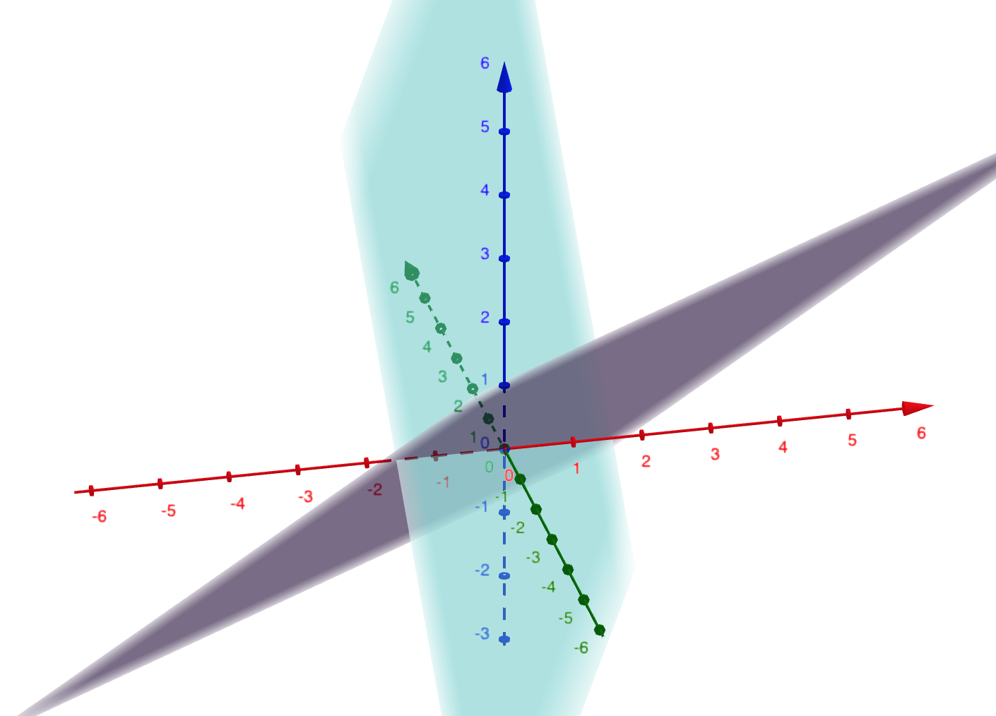
\[X = \begin{bmatrix} 1 & 1 \\ 1& 3 \\ 1 & -1\end{bmatrix}\]This is transforming \(\mathbb{R}^2\) into a plane in \(\mathbb{R}^3\). It does so in a way which distorts both angles and distances. The angle and distance between two vectors before the transformation will not be the same as their angle and distance after. \(X^\top X\) is a tool which helps us understand how these angles and distances are distorted! We are thinking of \(X^\top X\) as a bilinear form \(\mathbb{R}^p \times \mathbb{R}^p \to \mathbb{R}\) mapping \((\vec{\beta}_1, \vec{\beta}_2) \mapsto \vec{\beta}_2^\top X^\top X \vec{\beta}_1 = \langle X \vec{\beta}_1, X \vec{\beta}_2\rangle\).
Please play with this geogebra app:
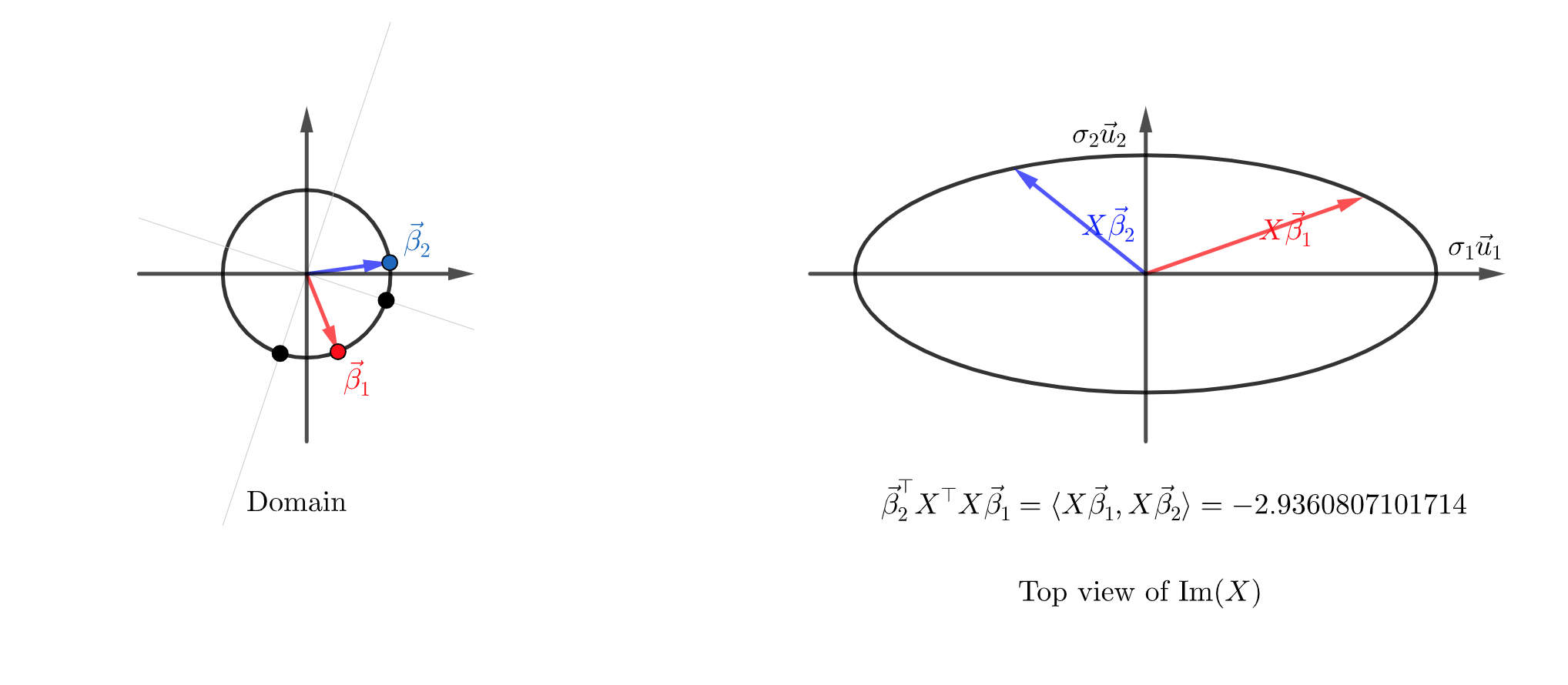
Here we can see two vectors \(\vec{\beta}_1\) and \(\vec{\beta}_2\) in the domain. I am looking at their image in the codomain (which is 3 dimensional), but looking “straight down” in the direction of \(\vec{u}_3\). Essentially I just picked up \(\textrm{Im(X)}\) and plopped it down flat on the page so that \(\vec{u}_1\) was in the positive \(x\) direction, and \(\vec{u}_2\) was in the positive \(y\) direction.
We can see the both the angle between the inputs and the length of the inputs have changed.
Thinking of \(X^\top X \vec{\beta}_1\) as living in the same space as \(\vec{\beta}_1\) leads to some confusion. Even though these have the same dimensions, it might really be better to think of \(X^\top X \vec{\beta}_1\) as covector than as a vector. It is a partially applied version of the bilinear form we discussed above. In other words, you should be thinking of \(X^\top X \vec{\beta}_1\) as a map \(\mathbb{R}^p \to \mathbb{R}\) defined by \(\vec{\beta}_2 \mapsto \vec{\beta}_2^\top X^\top X \vec{\beta}_1 = \langle X \vec{\beta}_1, X \vec{\beta}_2\rangle\). You might recognize that from this perspective, \(X^\top X \vec{\beta}_1\) is a curried form of \(X^\top X\) viewed a bilinear form.
Nonetheless, we can view \(X^\top X \vec{\beta}\) as a vector, and the nicest way to visualize it is probably by thinking of it as (a multiple of) the gradient of the map \(\vec{\beta} \mapsto \vert X\vec{\beta}\vert^2\). We can then levarage our intuition about gradient vectors pointing in the direction of greatest increase, being perpendicular to level sets, and having magnitude representing the “steepness” of ascent.
Play around with this geogebra app:
The standard Lagrange multiplier intuition shows us why the \(\vec{\beta}\) which maximizes \(\vert X\vec{\beta}\vert^2\) must be an eigenvector for \(X^\top X\).
I think that our understanding of \(X^\top X\) as a bilinear form is the most important take away from this section though. We will see how this is crucial to understanding how SVD gives us optimal low rank approximations of a matrix.
Using SVD to project onto a subspace
Remember that we defined \(r = \textrm{Rank}(X)\) and \(U_r\) to be the first \(r\) columns of \(U\).
The columns of \(U_r\) form an orthonormal basis of the image of \(X\). So it is easy to use it to project a vector \(\vec{y}\) onto the image of \(X\):
\[\hat{y} = \text{Proj}_{\textrm{Im}(X)} (\vec{y}) = \sum_1^r (\vec{y} \cdot \vec{u}_j) \vec{u_j}\]This can be rewritten as a matrix product as
\[\hat{y} = U_{r} U_{r}^\top \vec{y}\]To find the value of \(\beta\) with \(\hat{y} = X \vec{\beta}\), we can use
\[\begin{align*} X \beta &= U_{r} U_{r}^\top \vec{y}\\ U_{r} \Sigma_r V_r^\top \beta &= U_{r} U_{r}^\top \vec{y}\\ \Sigma_r V_r^\top \beta &= U_{r}^\top \vec{y}\\ V_r^\top \beta &= \Sigma_r^{-1} U_{r}^\top \vec{y}\\ \beta &= V_r \Sigma_r^{-1} U_{r}^\top \vec{y} \end{align*}\]This should make intuitive sense as well:
- When we orthogonally project \(\vec{y}\) onto the image of \(X\), \(U_{r}^\top \vec{y}\) gives the coefficients of the \(\vec{u}_j\) spanning the image. Say
Then
\[U_{r}^\top \vec{y} = \begin{bmatrix} c_1 \\ c_2 \\ \vdots \\ c_r \end{bmatrix}\]- So \(\Sigma_r^{-1} U_{r}^\top \vec{y}\) is scaling each of these coefficients by \(\frac{1}{\sigma_j}\):
- Finally \(\beta = V_r \Sigma_r^{-1} U_{r}^\top \vec{y}\) takes the linear combination of the right singular vectors \(\vec{v}_j\) using these coefficients.
\(\beta = \frac{c_1}{\sigma_1} \vec{v}_1 + \frac{c_2}{\sigma_2} \vec{v}_2 + \dots + \frac{c_r}{\sigma_r} \vec{v}_r\)
- Applying \(X\) to \(\beta\) will return \(\hat{y}\) since
We can use this for linear regression!
Let’s check using some synthetic data:
import numpy as np
import pandas as pd

ones = np.ones((100,1))
x1 = np.random.random((100,1))
x2 = np.random.random((100,1))
X = np.stack([ones, x1, x2], axis = 1).reshape((100,3))

y = 2*ones - x1 + 3*x2 + np.random.normal(0,0.1,(100,1))

from sklearn.linear_model import LinearRegression
reg = LinearRegression(fit_intercept = False).fit(X, y) # X has a column of ones, so I set fit_intercept = False.
y_hat_sklearn = reg.predict(X)

svd_stuff = np.linalg.svd(X)
    # Note np.linalg.svd(X) is a tuple (U, list of singular values, V^\top)
U = svd_stuff[0]
U_r = U[:,:3] # The image is 3 dimensional, so we the first 3 left singular vectors span the image.
y_hat_svd = np.dot(np.dot(U_r, np.transpose(U_r)), y) # projecting onto the image using the first 3 left singular vectors

print((y_hat_sklearn - y_hat_svd).max()) # This should be close to 0!
4.440892098500626e-16
S_r = np.diag(svd_stuff[1])
S_r_inv = np.linalg.inv(S_r) # Note:  this is easy to calculate.  Just 1 divided by each singular value.
V_r = np.transpose(svd_stuff[2])[:,:3]
beta_svd = np.dot(np.dot(V_r, np.dot(S_r_inv, np.transpose(U_r))), y)
print('These should agree: \n', beta_svd, '\n\n',  reg.coef_)
These should agree: [[ 2.01228328] [-1.01411842] [ 2.98989642]]
[[ 2.01228328 -1.01411842 2.98989642]]
Using SVD to find low rank approximations of a matrix
Note: I learned this story about variational characterizations originally from Qiaochu Yuan’s blog, which is also an excellent take on all of this SVD content. They are more terse and less geometric in their exposition.
To understand how SVD gives low rank approximations, we should first understand the following two variational approach to the singular vectors and values:
Theorem: (First Variational Characterization of singular values)
Let \(X\) be an \(n \times p\) matrix. Let \(j \in \{1,2,3,...,p\}\).
We can characterize \(\sigma_j\) as follows:
\[\sigma_j = \max_{\substack{ V \subset \mathbb{R}^p \\ \textrm{dim}(V) = j}} \min_{\substack{ \vec{v} \in V \\ \vert\vec{v}\vert = 1}} \vert M \vec{v}\vert\]In other words, to find \(\sigma_j\) we look at all subspaces of dimension \(j\) of the domain, minimize \(\vert M \vec{v}\vert\) over the unit ball in that subspace. Different subspaces give us different minimum values. We choose the subspace \(V\) which maximizes this minimum value. In that case, the minimum value is \(\sigma_j\).
If you have been following along, this should not be a surprizing characterization!
Here is the proof.
We already know that \(V_{\textrm{svd}} = \textrm{Span}(\vec{v}_1, \vec{v}_2, \vec{v_3}, ... \vec{v_j})\) we have
\[\min_{\substack{ \vec{v} \in V_{\textrm{svd}} \\ \vert\vec{v}\vert = 1}} \vert M \vec{v}\vert = \sigma_j\]This is true just by construction of the right singular vectors.
We need to show that any other choice of \(V\) gives us a smaller result than \(\sigma_j\).
Let \(V'\) be another subspace of dimension \(k\).
Then \(\textrm{Span}(v_j, v_{j+1}, ..., v_{p})\) is a \(p-j+1\) dimensional subspace, the intersection of \(V'\) with this subspace must be at least \(1\) dimensional. Take a unit vector \(\vec{v} \in V' \cap \textrm{Span}(v_j, v_{j+1}, ..., v_{p})\). Let
\[\vec{v} = \sum_{i=j}^{i=p} c_i \vec{v}_i \textrm{ with } \sum_{i=j}^{i=p} \vert c_i\vert^2 = 1\]Then
\[\begin{align*} \vert X \vec{v}\vert^2 &= \left\vert \sum_{j}^p X(c_i \vec{v}_i)\right\vert^2\\ &= \left\vert \sum_{j}^p c_i \sigma_i \vec{u}_i \right\vert^2\\ &= \sum_{j}^p (\vert c_i\vert^2 \vert\sigma_i\vert^2) \textrm{ Pythagorean Theorem: $\vec{u}_i$ are orthogonal!}\\ &\leq \sum_{j}^p (\vert c_i\vert^2 \vert\sigma_j\vert^2) \textrm{ since $\sigma_j \geq \sigma_{j+1} \geq ...$}\\ &= \vert\sigma_j\vert^2 \sum_{j}^p (\vert c_i\vert^2 )\\ &= \vert\sigma_j\vert^2 \end{align*}\]as desired!
Theorem: (Second Variational Characterization of singular values)
Let \(X\) be an \(n \times p\) matrix. Let \(j \in \{1,2,3,...,p\}\).
We can characterize \(\sigma_{j+1}\) as follows:
\[\sigma_{j+1} = \min_{\substack{ V \subset \mathbb{R}^p \\ \textrm{dim}(V) = p-j}} \max_{\substack{ \vec{v} \in V \\ \vert\vec{v}\vert = 1}} \vert M \vec{v}\vert\]Here is the (very similar!) proof:
We already know that for \(V_{\textrm{svd}} = \textrm{Span}(\vec{v}_{j+1}, \vec{v}_{j+2}, \vec{v_{j+3}}, ... \vec{v_p})\) we have
\[\max_{\substack{ \vec{v} \in V_{\textrm{svd}} \\ \vert\vec{v}\vert = 1}} \vert M \vec{v}\vert = \sigma_{j+1}\]This is true just by construction of the right singular vectors.
We need to show that any other choice of \(V\) gives us a larger result than \(\sigma_{j+1}\).
Let \(V'\) be another subspace of dimension \(p-j\).
Then \(\textrm{Span}(v_1, v_2, ..., v_j, v_{j+1})\) is a \(j+1\) dimensional subspace, the intersection of \(V'\) with this subspace must be at least \(1\) dimensional. Take a unit vector \(\vec{v} \in V' \cap \textrm{Span}(v_1, v_2, ..., v_j, v_{j+1})\). Let
\[\vec{v} = \sum_{i=1}^{i=j+1} c_i \vec{v}_i \textrm{ with } \sum_{i=1}^{i=j+1} \vert c_i\vert^2 = 1\]Then
\[\begin{align*} \vert X \vec{v}\vert^2 &= \left\vert \sum_{1}^{j+1} X(c_i \vec{v}_i)\right\vert^2\\ &= \left\vert \sum_{1}^{j+1} c_i \sigma_i \vec{u}_i \right\vert^2\\ &= \sum_{1}^{j+1} (\vert c_i\vert^2 \vert\sigma_i\vert^2) \textrm{ Pythagorean Theorem: $\vec{u}_i$ are orthogonal!}\\ &\geq \sum_{1}^{j+1} (\vert c_i\vert^2 \vert\sigma_{j+1}\vert^2) \textrm{ since $\sigma_1 \geq \sigma_{2} \geq ... \geq \sigma_{j+1}$}\\ &= \vert\sigma_{j+1}\vert^2 \sum_{1}^{j+1} (\vert c_i\vert^2 )\\ &= \vert\sigma_{j+1}\vert^2 \end{align*}\]as desired!
We are now ready for:
Theorem (Low rank approximation)
Let \(X\) be an \(n \times p\) matrix. Let \(X = U \Sigma V^\top\) be an SVD decomposition. Let \(\Sigma_j\) be the \(n \times p\) matrix with diagonal values
\[\Sigma_{k,k} = \begin{cases}\sigma_k \textrm{ if $k \leq j$} \\ 0 \textrm{ else}\end{cases}\]Let \(X_j = U \Sigma_j V^\top\). Clearly \(\textrm{Rank}(X_j) \leq j\) (with equality if \(\sigma_j \neq 0\)).
Our claim is that the \(X_j\) is the matrix of rank at most \(j\) which is closest to \(X\) in operator norm, and this minimal value is \(\sigma_{j+1}\). The operator norm of a matrix \(M\) is largest singular value of \(M\) (aka the maximum value of \(\vert M\vert\) on the unit sphere).
Proof:
Let \(M_j\) be any other matrix of rank at most \(j\). Then \(\textrm{Null}(M_j)\) has dimension at least \(p-j\). By the second variational characterization, there must be a unit vector \(\vec{v} \in \textrm{Null}(M_j)\) with \(\vert X \vec{v}\vert \geq \sigma_{j+1}\). But \(\vert X \vec{v}\vert = \vert X\vec{v} - M_k\vec{v}\vert\) since \(M_k\vec{v} = 0\). Hence the operator norm of \(X - M_k\) is at least \(\sigma_{j+1}\).
On the other hand \(X - X_j = U (\Sigma - \Sigma_k) V^\top\). This is the SVD decomposition of \(X - X_j\) (up to reordering of the columns to put the singular values in descending order). So we can see that largest singular value of this matrix is \(\sigma_{j+1}\), which is its operator norm.
Principle angles between subspaces
You are probably familiary with the fact that the angle between two vectors \(\vec{u}\) and \(\vec{v}\) can be defined as
\[\theta(u,v) = \angle(u, v) = \arccos\left( \frac{\vert \langle \vec{u}, \vec{v}\rangle \vert}{\vert\vec{u} \vert \vert \vec{v}\vert}\right)\]You can probably also work out ad-hoc defininitions for the angle between a \(1\)-dimesional subspace and a \(2\)-dimensional subspace, or the angle between two \(2\)-dimensional subspaces.
In higher dimensions things get a bit tougher. If you have an \(i\) and \(j\) dimensional subspace of \(\mathbb{R}^d\), a single “angle” is no longer suitable as a description of the relationship between these subspaces.
In this section we motivate the definition of the principle angles between two subspaces, and prove that these angles can be computed using the SVD of a certain matrix. This will give a beautiful geometric interpretation for the subspace similarity measurement introduced in the LoRa paper (which we will cover in the next, final, section).
We quote Wikipedia’s variational definition (adjusting the notation to fit our use case) since it is the closest in spirit to the kind of work we have been doing, and (imho) is also the most geometrically motivated definition:
Given two subspaces \(\mathcal{U},\mathcal{W}\) of \(\mathbb{R}^d\) with \(\dim(\mathcal{U})=i \leq \dim(\mathcal{W}):=j\), there exists then a sequence of \(i\) angles \(0 \le \theta_1 \le \theta_2 \le \cdots \le \theta_k \le \pi/2\) called the principal angles, the first one defined as:
\[\theta_1:=\min \left\{ \arccos \left( \frac{ \vert \langle u,w\rangle\vert}{\vert u \vert \vert w \vert }\right) \,: \, u\in \mathcal{U}, w\in \mathcal{W} \right\}=\angle(u_1,w_1),\]The vectors \(u_1\) and \(w_1\) are the corresponding ‘‘principal vectors.’’
The other principal angles and vectors are then defined recursively via:
\[\theta_i:=\min \left\{ \arccos \left( \frac{ \vert \langle u,w\rangle\vert }{\vert u \vert \vert w \vert }\right) \,: \, u\in \mathcal{U},~w\in \mathcal{W},~u\perp u_j,~w \perp w_j \quad \forall j\in \{1,\ldots,i-1\} \right\}.\]This means that the principal angles \((\theta_1,\ldots, \theta_k)\) form a set of minimized angles between the two subspaces, and the principal vectors in each subspace are orthogonal to each other.
Let’s see how this is connected with the SVD.
Let \(U\) be a \(d \times i\) matrix whose columns are orthonormal and span \(\mathcal{U}\). Similarly, let \(W\) be a \(d \times j\) matrix whose columns are orthonormal and span \(\mathcal{W}\).
Consider the matrix \(P = W W^\top U\). Let \(\beta\) be a unit vector in \(\mathbb{R}^i\). Then \(U\vec{\beta}\) is a unit vector on \(\mathcal{U}\) since
\[\begin{align*} \vert U\vec{\beta}\vert^2 &= \langle U\vec{\beta}, U \vec{\beta}\rangle \\ &= \langle \vec{\beta}, U^\top U \vec{\beta}\rangle \\ &= \langle \vec{\beta}, \mathbb{I}_i \vec{\beta}\rangle \\ &= \langle \vec{\beta}, \vec{\beta}\rangle \\ &= \vert \vec{\beta}\vert^2\\ &= 1 \end{align*}\]\(P \vec{\beta}\) computes the orthogonal projection of the unit vector \(\vec{u} = U \vec{\beta}\) onto the subspace \(\mathcal{W}\). Why? Let the columns of \(W\) be called \(\vec{w}_k\). Then
\[\begin{align*} P\vec{\beta} &= W W^\top \vec{u}\\ &= W W^\top \vec{u}\\ &= \sum_1^j \vec{w}_k (\vec{w}_k^\top \vec{u})\\ &= \sum_1^j \langle \vec{u}, \vec{w}_k \rangle \vec{w}_k\\ \end{align*}\]This is the sum of the projections of \(\vec{u}\) into the direction of each of the orthonormal \(\vec{w}_k\).
We will now see the connection between the singular value decomposition of this projection matrix with the principle angles.
Since we have already used \(U\), I will write the singular value decomposition as:
\[P = T \Sigma V\]A few obervations:
- We saw that \(U\) is length preserving, and since \(W^\top W\) is an orthogonal projection it satisfies \(\vert W^\top W \vec{u}\vert \leq \vert \vec{u}\vert\) (this is a consequence of the Pythagorean theorem!). So \(P\) also satisfies \(\vert P(\vec{u}) \vert < \vert \vec{u}\vert\).
- As a consequence of this, the singular values of \(P\) are all in the interval \([0,1]\).
Let’s look again at the definition of the first principle angle:
\[\theta_1:=\min \left\{ \arccos \left( \frac{ \vert \langle u,w\rangle\vert}{\vert u \vert \vert w \vert }\right) \,: \, u\in \mathcal{U}, w\in \mathcal{W} \right\}\]
Since the \(\arccos\) function is decreasing, we can rewrite this as
\[\cos(\theta_1):=\max \left\{ \frac{ \vert \langle u,w\rangle\vert}{\vert u \vert \vert w \vert } \,: \, u\in \mathcal{U}, w\in \mathcal{W} \right\}\]
by bilinearity we can scale \(\vec{u}\) and \(\vec{w}\) by any non-zero constant without changing \(\frac{ \vert \langle u,w\rangle\vert}{\vert u \vert \vert w \vert }\). So we can instead maximize over the vectors of unit length:
\[\cos(\theta_1):=\max_{\substack{ \vert \vec{u}\vert = 1 \\ \vert\vec{w}\vert = 1 \\ }} \left\{ \vert \langle u,w \rangle \vert : \, u \in \mathcal{U}, w\in \mathcal{W} \right\}\]
There is a unique unit vector \(\beta \in \mathbb{R}^i\) with \(U\beta = \vec{u}\), and \(w\) is the unique unit vector in \(\mathbb{R}^d\) with \(w = W W^\top w\). Thus \(\langle u,w \rangle = \langle U \beta, W W^\top w \rangle = \langle W W^\top U \beta, w \rangle = \langle P \beta, w \rangle\).
Since \(w\) and \(P \beta\) are both in \(\mathcal{W}\), their dot product will be maximized when they point in the same direction (except in the special case \(P \beta = 0\)). So the maximum values of \(\langle P \beta, w \rangle\) is equal to \(\vert P \beta \vert\) where the maximum is taken over the unit sphere in \(\mathbb{R}^i\):
\[\cos(\theta_1):=\max_{\vert \vec{\beta}\vert = 1} \left\{ \vert P \beta \vert : \, \beta \in \mathbb{R}^i \right\}\]
This was our definition of the first singular value of \(P\), so we have:
Lemma: \(\cos(\theta_1)\) is the first singular value of the projection matrix \(P = WW^\top U\).
An identical analysis (just follow our inductive construction of the SVD process) gives us the theorem:
Theorem: \(\cos(\theta_k) = \sigma_k\) where \(\sigma_k\) are the singular values of the projection matrix \(P = WW^\top U\).
Whew!
Let’s try to visualize this to get a bit more geometric intuition.
Consider the two planes \(\mathcal{U}\) and \(\mathcal{W}\) spanned by the columns matrices
\[U = \begin{bmatrix} 1 & 1\\ 2 & 5\\ -1 & 6 \end{bmatrix} \hphantom{dsds} W = \begin{bmatrix} 1 & 3 \\ -1 & 2\\ 2 & 0 \end{bmatrix}\]
We visualize the unit circle in \(\mathcal{U}\) and its orthogonal projection on onto \(\mathcal{W}\), which is an ellipse:
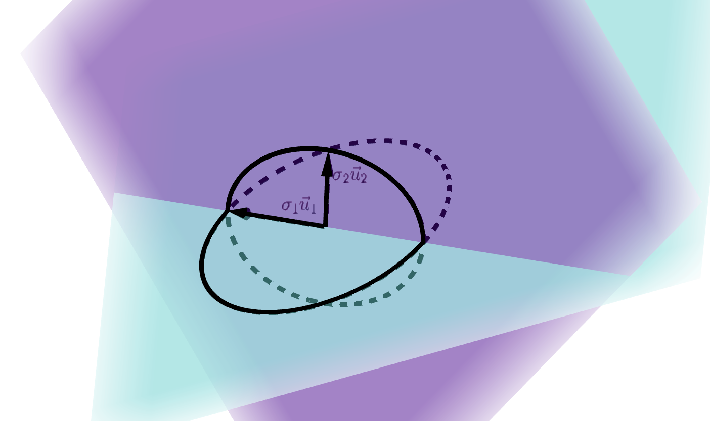
Since these planes intersect, the longest length of an orthogonal projection of a unit vector from \(\mathcal{U}\) onto \(\mathcal{W}\) will be \(1\): these vectors actually coincide! So the first left singular vector of \(W^\top W U\) would be a unit vector which lies in this intersection, the first left singular value would be \(1\), and the first principle angle would be \(0\).
The next second singular vector would be a unit vector pointed in the direction of the minor axis of the ellipse in \(\mathcal{W}\). The second singular value is the distance from the origin to that vertex. The second principle angle would be be the inverse cosine of that distance. Make sure you understand why this is “exactly what you want” geometrically: \(\sigma_2 \vec{u}_2\) is the base of a right triangle whose hypotenuse is a vector on the unit circle in \(\mathcal{U}\)!
The subspace similarity metric in the LoRa paper.
We are now finally ready to understand the similarity metric introduced in the LoRa paper. I quote:
In this paper we use the measure \(\phi(A,B,i,j) = \psi (U_A^i, U_B^j) = \frac{\vert(U_A^i)^\top U_B\vert^2_F}{\min \{i,j\}}\) to measure the subspace similarity between two column orthogonal matrices \(U_A^i \in \mathbb{R}^{d \times i}\) and \(U_B^j \in \mathbb{R}^{d \times j}\), obtained by taking columns of the left singular matrices of \(A\) and \(B\).
Note that there is a typo in the paper. I am quite sure that they meant to write \(\frac{\vert(U_A^i)^\top U_B^{j}\vert^2_F}{\min \{i,j\}}\) [note the “j” in the “exponent” of \(U_B^j\)].
Let’s break this down!
Let \(C\) be a \(d \times p\) matrix with SVD \(C = U_C \Sigma_C V_C^\top\).
In their notation, \(U_C^k\) would be the matrix obtained by only retaining the first \(k\) columns of \(U\). Let \(C_k\) be the best rank at most \(k\) approximation of \(C\) with respect to the operator norm. By the results in the last section, we know that the column space of \(U_C^k\) is the image of \(C_k\)!
So comparing the subspaces \(U_A^i\) and \(U_B^j\) is a very reasonable thing to do. We wouldn’t want to use all of \(U_A\) and \(U_B\) because the column space of both of those is all of \(\mathbb{R}^d\)! We could use \(U_A^\textrm{Rank(A)} = \textrm{Im}(A)\) and \(U_B^\textrm{Rank(B)} = \textrm{Im}(B)\), but the reality is that (as we have seen) it is the left singular vectors with the largest singular values which carry “most of the information” about a matrix. The low singular values correspond to noise. This is the intuitive content of our low rank approximation result. So it makes sense that instead of taking all of the non-negative singular values, we might only want to retain the top “so many” of them. This is what \(U_A^i\) and \(U_B^j\) are doing: they are retaining the \(i\) (respectively \(j\)) most important left singular vectors.
Now \((U_A^i)^\top U_B^{j}\) looks an awful lot like the projection matrix \(U_A^i (U_A^i)^\top U_B^{j}\) we met in the last section on principle angles! In fact, these two matrices will have the same singular values (since, as we have computed, \(\vec{v} \mapsto M \vec{v}\) is a distance preserving map when the columns of \(M\) are orthonormal, as is the case for \(U_A^i\)).
They are using the Frobenius norm of this matrix. We really just need to know the definition:
\[\vert A \vert_\text{F} = \sqrt{\sum_{i}^m\sum_{j}^n \vert a_{ij}\vert ^2} = \sqrt{\operatorname{trace}\left(A^* A\right)} = \sqrt{\sum_{i=1}^{\min\{m, n\}} \sigma_i^2(A)}\]A couple nice things about this norm:
- It is much easier to compute than the operator norm. We don’t actually need to find the singular values of \(A\), as the first two formulas show.
- Even so, it carries information about all of the singular values of \(A\).
Note: it is a nice exercise to prove the equivalence of these three ways of computing the norm. If you have been working through everything so far it shouldn’t be out of your reach to prove this.
Given the results of the last section, we can rewrite the similarity measure using the more “geometric” language of principle angles:
\[\phi(A,B,i,j) = \frac{1}{\min\{m, n\}}\sum_{i=1}^{\min\{m, n\}} \cos^2(\theta_i)\]where \(\theta_i\) are the principle angles between the columns spaces of \(U_A^i\) and \(U_B^j\).
In words, we are taking the “mean of the squared cosines of the principle angles”, where we are only averaging over the smaller of the two dimensions of the subspaces.
Armed with this intuitive perspective several things become obvious:
- The maximum value of \(\phi(A,B,i,j)\) is \(1\), and this is only achieved when the smaller subspace is contained in the larger one.
- The minimum value of \(\phi(A,B,i,j)\) is \(0\), and this is only achieved when the smaller subspace is in the orthogonal complement of the larger one.
I hope that this similarity measure makes a lot more sense to you now!