Explaining the Model
We will explain fitting logistic regression using a toy example. A standard apple tree which is only \(1\) foot tall is unlikely to bear fruit this year. However an apple tree which is \(20\) feet tall is very likely to be of bearing age. We might expect an increasing relationship between the height of the tree and the probability that the tree is capable of bearing fruit.
import numpy as np
import pandas as pd
import math
import matplotlib.pyplot as plt
height_vs_bearing = pd.read_csv('height_vs_bearing.csv', index_col=0)
height_vs_bearing
| height | bearing | |
|---|---|---|
| 0 | 11.325206 | 0.0 |
| 1 | 12.939280 | 1.0 |
| 2 | 9.767215 | 1.0 |
| 3 | 7.638947 | 0.0 |
| 4 | 8.997293 | 0.0 |
| ... | ... | ... |
| 95 | 12.316341 | 1.0 |
| 96 | 8.523462 | 0.0 |
| 97 | 7.432771 | 0.0 |
| 98 | 7.105060 | 0.0 |
| 99 | 7.487725 | 0.0 |
100 rows × 2 columns
We can see that we have measured the height of 100 apple trees, and recorded whether or not the tree is currently bearing apples.
Here is a graph of the data:
X = height_vs_bearing['height']
y = height_vs_bearing['bearing']
plt.figure(figsize=(6,5))

plt.scatter(X, y)

plt.xlabel("$X$", fontsize=12)
plt.ylabel("$y$", fontsize=12)
plt.show()
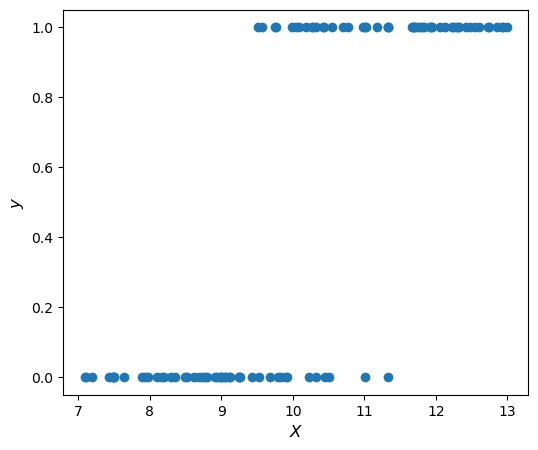
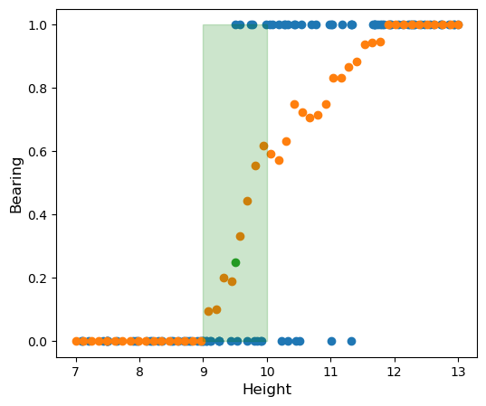
As we can see, when the tree is shorter than 9 feet tall it is very rare for it to bear apples. When it is taller than 11.5 feet tall it is almost surely going to bear apples. In between we have a murkier situation. One thing we could do to try to get a better understanding of this relationship is try and see how the probability of bearing varies as a function of height. We can estimate the probability \(P(\textrm{bearing} = 1 \vert x )\) by looking at the empirical probability of bearing in a small neighborhood of \(x\), say
\[P(\textrm{bearing} = 1 \vert \textrm{height} = x ) \approx \frac{\textrm{# samples bearing}}{\textrm{# samples in }[x-0.5,x+0.5]}\]Let’s take a look at that graph. I have highlighted the point with \(\textrm{height} = 9.5\) green. In the interval \([9,10]\) there are \(20\) samples of which \(5\) are bearing, for an estimated probability of \(\frac{5}{20} = 0.25\)
We would like to model the probability as a funtion of height directly. Our model might look something like this:
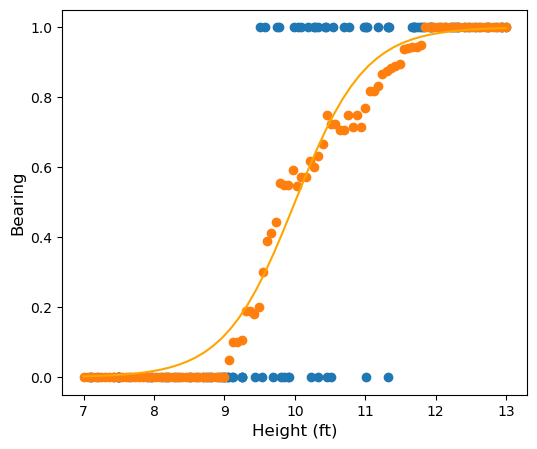
In logistic regression we will model the probability \(P(\textrm{bearing} = 1\vert \textrm{height} = x)\) using a function of the form \(p(x) = \sigma(mx+b)\) where \(\sigma\) is the sigmoid function defined by
\[\sigma(t) = \frac{1}{1+e^{-t}}\]We can interpret this as follows
\[\begin{align*} &p(x) = \frac{1}{1+e^{-(mx+b)}}\\ &\frac{1}{p(x)} = 1 + e^{-(mx+b)}\\ &\frac{1 - p(x)}{p(x)} = e^{-(mx+b)}\\ &\frac{p(x)}{1-p(x)} = e^{mx+b}\\ &\log\left(\frac{p(x)}{1-p(x)}\right) = mx+b \end{align*}\]The quantity \(\frac{p(x)}{1-p(x)}\) is the odds in favor of bearing.
So by modeling our probability using the parameteric family \(p(x) = \sigma(mx+b)\) we are making the assumption that the log-odds in favor of bearing is approximately linear in the height. In other words, we are assuming that each foot of height increases the log-odds in favor of bearing by a fixed amount (\(m\)). This assumption may or may not be reasonable, just like fitting a linear regression may or may not be reasonable. In this case our exploratory plot makes it look like a reasonable model.
Fitting the Model
As explained in Understanding Binary Cross-entropy , we are going to fit this model by minimizing the binary cross-entropy
\[\ell(m,b) = -\sum_{i = 1}^N y_i\log(p_{m,b}(x_i)) + (1- y_i)\log(1- p_{m,b}(x_i))\]We are going to find the gradient of this loss function. Before that, it is convenient to note a few special properties of the sigmoid function:
- \(1 - \sigma(z) = -\sigma(z)\)
- \(\frac{\sigma(z)}{\sigma(-z)} = \sigma(z)\)
- \(\frac{\textrm{d}}{\textrm{d}z} \sigma(z) = \sigma(z) \sigma( - z)\)
These properties are all elementary to derive, so we skip the derivations.
We first use these properties to rewrite the loss function in a more convenient form:
\[\begin{align*} \ell(m,b) &= -\sum_{i = 1}^N y_i\log(p_{m,b}(x_i)) + (1- y_i)\log(1- p_{m,b}(x_i))\\ & = -\sum_{i=1}^n y_i \log(\sigma(mx_i+b)) + (1- y_i)\log(1- \sigma(mx_i + b))\\ & = -\sum_{i=1}^n y_i \log(\sigma(mx_i+b)) + (1- y_i)\log(\sigma(-(mx_i + b))) \textrm{ by 1.}\\ & = -\sum_{i=1}^n y_i \log(\frac{\sigma(mx_i + b)}{\sigma(-mx_i + b)}) + \log(\sigma(-(mx_i + b)))\\ & = -\sum_{i=1}^n y_i \log(e^{mx_i+b}) + \log(\sigma(-(mx_i + b))) \textrm{ by 2.}\\ & = -\sum_{i=1}^n y_i(mx_i + b) + \log(\sigma(-(mx_i + b))) \textrm{ by 2.}\\ \end{align*}\]Side note: It is interesting to me that \(-\log(\sigma(-z)) = \log(1 + e^z) \approx \textrm{relu}(z)\) (for large \(\vert z\vert\)) is making an appearance here.
We are now in a strong position to take partial derivatives:
\[\begin{align*} \frac{\partial \ell}{\partial b} &= -\sum_{i=1}^n y_i - \frac{1}{\sigma(-(mx_i + b))} \sigma(-(mx_i + b))\sigma( mx_i + b) \textrm{ by 3.}\\ &= \sum_{i=1}^n \sigma( mx_i + b) - y_i \\ & = \sum_{i=1}^n p_{m,b}(x_i) - y_i \\ \end{align*}\] \[\begin{align*} \frac{\partial \ell}{\partial m} &= -\sum_{i=1}^n y_ix_i + -x_i \frac{1}{\sigma(-(mx_i + b))} \sigma(-(mx_i + b))\sigma( mx_i + b)\\ & = \sum_{i=1}^n x_i (p_{m,b}(x_i) - y_i) \\ \end{align*}\]It is amazing to me that these partial derivatives up having such (relatively) simple expressions!
If we package things a little differently the formula becomes even more compact.
Let
\[X = \begin{bmatrix} \vec{1} & \vec{x}\end{bmatrix} \hphantom{dsds} \vec{\beta} = \begin{bmatrix} b \\ m\end{bmatrix}\]Then it is easy to check that
\[\nabla \ell = X^\top (p_{\vec{\beta}}(\vec{x}) - \vec{y})\]To minimize the loss function we need to find where the gradient vanishes. Unfortunately, we cannot solve this analytically. We will instead resort to numerical approximation. We will use gradient descent.
import math

def sigma(z):
    return 1/(1 + math.exp(-z))

def loss(m,b):
    probs = (m*X+b).apply(sigma)  #applying sigma to mX+b to get the vector of predicted probabilities.
    return np.dot(y, np.log(probs)) + np.dot(1-y, 1 - np.log(probs)) # This is the formula for log-loss

def loss_grad(m,b):
    probs = (m*X+b).apply(sigma)
    partial_b = (probs - y).sum() #formula for partial derivative with respect to b from above
    partial_m = np.dot(X, probs - y) #formula for partial derivative with respect to m from above
    return np.array([partial_m, partial_b])

def grad_descent(m_start, b_start, h, tolerance):
    m = m_start
    b = b_start
    #we adjust m and b by h times the gradient while the length of the gradient is greater than our tolerance.
    while np.linalg.norm(loss_grad(m,b)) > tolerance:
        m -= h*loss_grad(m,b)[0]
        b -= h*loss_grad(m,b)[1]
    return np.array([m,b])


#My initial guess of m = 2, b = -20 is an educated guess.  Looking at the rough sketch we made of the probability curve when we first started, it looks like
#we have an inflection point at around (10,0.5) with a slope of 2.  This gives m = 2 and b = -20 after a little fiddling.  I could have started with a random
#guess, and it would have just taken a little longer to converge.

optimal_params = grad_descent(2,-20, 0.001, 0.01)  #Note this is a very inefficient implementation, just to get the ideas across, and takes my computer 5 minutes to run.

print(optimal_params)
[ 2.31265146 -23.31613122]
In contrast to our gradient descent function, scikit-learn fits the model almost instantly! They are using some much more sophisticated numerical analysis. See the Broyden–Fletcher–Goldfarb–Shanno algorithm for more details.
from sklearn.linear_model import LogisticRegression
log_reg = LogisticRegression(penalty=None)

## fit the model
log_reg.fit(X.to_numpy().reshape(-1,1),y.to_numpy())

# Note: sklearn fits the model almost instantly!  They are using some much more sophisticated numerical analysis.  See

print(f'Our gradient descent function obtains the fit m = {optimal_params[0]} and b = {optimal_params[1]}')
print(f'sklearn obtains the fit m = {log_reg.coef_[0][0]} and b = { log_reg.intercept_[0]}')
print('These are pretty close!')
Our gradient descent function obtains the fit m = 2.3126514601218653 and b = -23.316131222960646
sklearn obtains the fit m = 2.3365932232309583 and b = -23.557813056425687
These are pretty close!
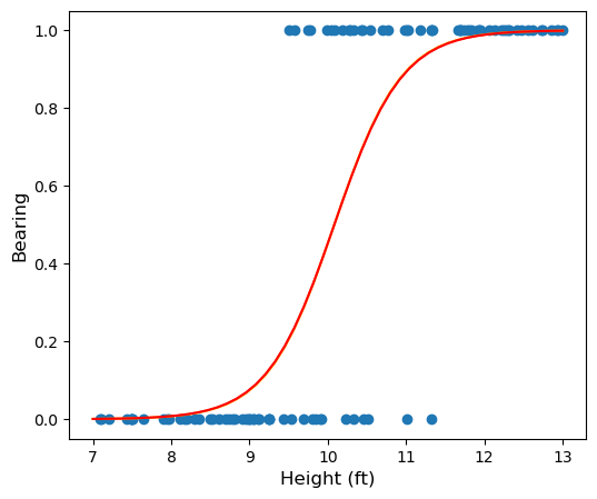
Let’s see how the fit generated by sklearn looks. You can check that the fit we obtained using gradient descent is indistinguishable to the human eye by uncommenting a line in the code below:
plt.figure(figsize=(6,5))

plt.scatter(X.to_numpy(), y.to_numpy())

sigmoid = lambda t: 1/(1+math.exp(-t))
plt.plot(np.linspace(7,13), np.vectorize(lambda x: sigmoid(log_reg.intercept_[0] + log_reg.coef_[0][0]*x))(np.linspace(7,13)), color = 'orange')
#plt.plot(np.linspace(7,13), np.vectorize(lambda x: sigmoid(optimal_params[1] + optimal_params[0]*x))(np.linspace(7,13)), color = 'red')

plt.xlabel("Height (ft)", fontsize=12)
plt.ylabel("Bearing", fontsize=12)
plt.show()
Uniqueness of Fit
When gradient descent converges it converges to a local minimum. It is possible that our loss function could have more than one local min. It turns out that when we are fitting logistic regression using cross-entropy loss the loss function is convex which ensures uniqueness of the global minimum (if it exists). We can show this by computing the Hessian matrix of the loss function and checking that it is positive definite. The Hessian matrix is
\[\begin{bmatrix} \frac{\partial^2 \ell}{\partial b^2} & \frac{\partial^2 \ell}{\partial b \partial m}\\ \frac{\partial^2 \ell}{\partial b \partial m} & \frac{\partial^2 \ell}{\partial m^2} \end{bmatrix}\]Let’s compute these partials:
\[\begin{align*} \frac{\partial^2 \ell}{\partial b^2} &= \frac{\partial}{\partial b} \sum_{i=1}^n p_{m,b}(x_i) - y_i\\ &= \frac{\partial}{\partial b} \sum_{i=1}^n \sigma(mx_i + b) - y_i\\ &= \sum_{i=1}^n \sigma(mx_i + b)\sigma( -(mx_i + b))\\ &\\ \frac{\partial^2 \ell}{\partial b \partial m} &= \frac{\partial}{\partial b} \sum_{i=1}^n x_i (p_{m,b}(x_i) - y_i)\\ &= \frac{\partial}{\partial b} \sum_{i=1}^n x_i( \sigma(mx_i + b) - y_i) \\ &= \sum_{i=1}^n x_i \sigma(mx_i + b)\sigma( -(mx_i + b)) &\\ \frac{\partial^2 \ell}{\partial m^2} &= \frac{\partial}{\partial m} \sum_{i=1}^n x_i (p_{m,b}(x_i) - y_i)\\ &= \frac{\partial}{\partial m} \sum_{i=1}^n x_i( \sigma(mx_i + b) - y_i) \\ &= \sum_{i=1}^n x_i^2 \sigma(mx_i + b)\sigma( -(mx_i + b)) \end{align*}\]This Hessian matrix can be written more compactly as
\[H = X^\top D X\]where \(D\) is the diagonal matrix with entires \(D_{ii} = \sigma(mx_i + b)\sigma( -(mx_i + b)) > 0\).
This allows us to easily see that the Hessian is positive semi-definite:
\[\begin{align*} \vec{v}^\top H \vec{v} &= \vec{v}^\top X^\top D X \vec{v}\\ &= (X \vec{v})^\top D (X \vec{v})\\ &\geq \textrm{min}_i(D_{ii}) \vert X \vec{v}\vert^2 \\ &\geq 0 \end{align*}\]Hence \(\ell\) is convex and has a unique global minimum (assuming that the global minimum exists). I will note that the minimum does exist as long as the data is not seperable, as explained in this stats.stackexchange answer.
Multiple logistic regression
Computing the gradient and Hessian for multiple logistic regression is harder, and requires us to be familiar with a bit more matrix calculus. I am writing this up here mostly because I have been unable to find a derivation of these formulas after a bit of googling, and I think it might be valuable to have it on the internet somewhere.
Set up:
We have \(k\) features \(x_1, x_2, ..., x_k\) and a binary response variable \(y\). We have a sample of \(N\) observations. The \(i^{th}\) observation has \(x_1 = x_{i1}, x_2 = x_{i2}, ... , x_k = x_{ik}\).
Let
\[\vec{x} = \begin{bmatrix} 1 & x_1 & ... & x_k \end{bmatrix}^\top\] \[\vec{\beta} = \begin{bmatrix} \beta_0 & \beta_1 & ... & \beta_k \end{bmatrix}^\top\]and
\[\vec{y} = \begin{bmatrix} y_1 & y_2 & y_3 ... & y_n\end{bmatrix}^\top\]We are modeling the probability that \(y = 1\) given the values \(\vec{x}\) for our features as
\[p_{\vec{\beta}}(\vec{x}) = \sigma(\vec{\beta} \cdot \vec{x})\]Introducing a bit more notation, let \(X\) be the \(N\) by \(k+1\) matrix
\[X = \begin{bmatrix} 1 & x_{11} & x_{12} & ... & x_{1k}\\ & & \vdots & & \\ 1 & x_{N1} & x_{N2} & ... & x_{Nk}\\ \end{bmatrix}\]In the following formula when we apply \(\log\) or \(\sigma\) to a vector or matrix, understand this as applying the function to each coordinate. \(\vec{1}\) stands for a vector of ones of the appropriate dimension. \(\textrm{diag}(\vec{v})\) is the square matrix whose diagonal is the vector \(v\) and \(\textrm{diag}(A)\) is the diagonal vector of the matrix \(A\). \(\odot\) is element-wise multiplication, \(\oslash\) is element-wise division.
We will fit this model by minimizing the binary cross-entropy.
\[\begin{align*} \ell(\vec{\beta}) &= - \left( \vec{y} \cdot \log(\sigma(X \vec{\beta})) + ( \vec{1} - \vec{y}) \cdot \log(1- \sigma(X \vec{\beta}))\right)\\ &=- \left( \vec{y} \cdot \log(\sigma(X \vec{\beta})) + ( \vec{1} - \vec{y}) \cdot \log(\sigma( -X \vec{\beta}))\right) \textrm{ since $1-\sigma(t) = \sigma(-t)$}\\ &= -\vec{y} \cdot \log(\sigma(X \vec{\beta})) + ( \vec{y} - \vec{1}) \cdot \log(\sigma( -X \vec{\beta})) \end{align*}\]We compute \(\nabla \ell\) as follows:
\[\begin{align*} \nabla \ell(\vec{\beta}) &= - X^\top \left( \vec{y} \oslash \sigma(X \vec{\beta}) \right) \odot \sigma(X \vec{\beta}) \odot \sigma(-X \vec{\beta}) - X^\top \left( ((\vec{y} - \vec{1}) \oslash \sigma(-X \vec{\beta})) \odot \sigma(-X\vec{\beta}) \odot \sigma(X \vec{\beta})\right)\\ &= -X^\top \left( \vec{y} \odot \sigma(X \vec{\beta}) + (\vec{y} - \vec{1}) \odot \sigma(X \vec{\beta}) \right)\\ &= -X^\top \left( \vec{y} \odot (\sigma(X \vec{\beta}) + \sigma(-X \vec{\beta})) - \sigma(X\vec{\beta})\right)\\ &= X^\top \left( \sigma(X\vec{\beta}) - \vec{y} \right) \textrm{ since $\sigma(t) + \sigma(-t) = 1$}\\ &= X^\top \left( p_{\vec{\beta}}(X) - \vec{y}\right) \end{align*}\]As a sanity check, note that this recovers the formula for the gradient of the loss function we obtained in simple logistic regression!
We now compute the Hessian:
\[\begin{align*} H &= \frac{\partial}{\partial \vec{\beta}} \left( X^\top \left( p_{\vec{\beta}}(X) - \vec{y}\right) \right)\\ &= \frac{\partial}{\partial \vec{\beta}} \left( X^\top \left( \sigma(X \vec{\beta}) - \vec{y}\right) \right)\\ &= X^\top D X \end{align*}\]where \(D\) is the diagonal matrix with entries \(\sigma'(X \vec{\beta}) = \sigma(X \vec{\beta}) \sigma(-X\vec{\beta})\).
This is clearly positive semidefinite, and so multiple logistic regression is also a convex optimization problem!